|
Electron Tomography - Methods
by Hall and Rice
doi:10.3908/wormatlas.9.18
Image Collection
Sample Thickness, Beam Damage and Shrinkage
Resolution
Automation of Image Acquisition
Image Alignment
Fiducial marker alignment methods
Fiducial-less alignment methods
3-D Tomogram Reconstruction
Back-projection Methods
Algebraic and Iterative Methods
Filling in the Missing Wedge
Stacking Tomograms in Three Dimensions
"Large" Tomograms
Calculating Tomogram Resolution
Reducing Noise in Tomograms
Tomogram Annotation
Software Tools
Image Collection
Sample Thickness, Beam Damage and Shrinkage
Electrons interact with the specimen in two different ways. Elastic collisions of electrons with the specimen occur when the electrons are deflected without energy loss as they pass through the specimen. These electrons are appropriately focused by the lenses in the electron microscope and therefore provide high-resolution information. Since these electrons impart little energy to the specimen, they cause virtually no radiation damage. Inelastic collisions, in contrast, do transfer energy to the specimen, and therefore cause radiation damage. Worse, inelastically scattered electrons are not focused properly by the microscope (due to their energy loss), and thus contribute to noise in the image.
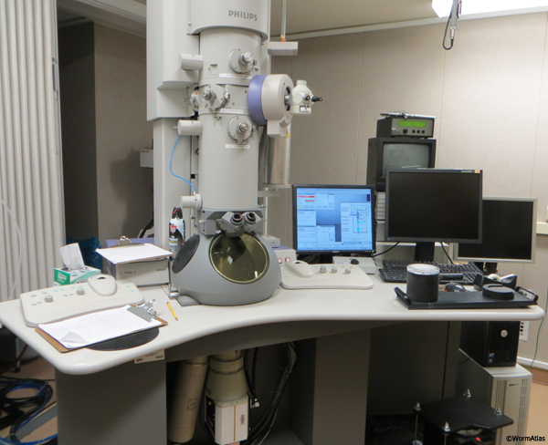
Very thick specimens will appear blurry because of the dominance of inelastically scattered electrons in the image. The use of an energy filter, which removes inelastically scattered electrons, can markedly improve the images of thick sections. In practice, we have found that specimens thicker than 200-250 nm are not suitable for high-tilt tomography on a 200 kV instrument (Tecnai F20) (ETFIG 1). Higher voltage (200 or 300kV) microscopes are desirable for tomography for two reasons. First, higher voltages provide better optics and allow thicker specimens to be imaged. Second, specimen damage decreases with increasing accelerating voltage, since higher voltage lowers the cross-section for scattering. However, for the same reason, images from a higher voltage microscope will have less contrast than those obtained from a lower voltage microscope. For this reason, when tilted to 70°, a 250 nm section will have an apparent depth of almost one micron, and cannot be viewed at less than 200 kV.
 Although resin-embedded and heavy metal stained biological sections are somewhat resilient to electron beam damage, they do change as they are exposed to the beam (Egerton et al., 2004). The most important and noticeable effect is specimen shrinkage, especially along the z-axis. Shrinkage occurs in two phases, fast and slow (Luther et al., 1988). Since reconstruction algorithms assume that only the tilt angle, and not the sample itself, is changing, it is important to minimize sample shrinkage during data collection. While it would be possible to use low-dose techniques for plastic sections, it is more common to pre-irradiate the samples before collection of tilt-series data. In this way, data is collected only during the slow phase (Luther et al., 1988). In practice, we usually set up scripts to collect images of the ROI before and after pre-irradiation. This allows for an estimation of shrinkage in the X-Y plane. We commonly dose to ~2000 e/A2 before collecting tilt series. It is important to dose a significantly larger area than the ROI, since outside areas will later enter the field of view at high tilt angles and become subject to fast shrinkage. Note that a full day (or night) of EM time may be needed for the pre-dosing step if many ROIs are to be collected.
Resolution
Electron Tomography is a technique that utilizes the TEMs large depth of field to study samples from 50-500 nm in thickness (from whole cells to suspensions of macromolecular complexes). The resolution of the resulting tomogram will depend on the specimen preparation, microscope conditions and image processing but is usually between 5 and 10 nm. The theoretical resolution can be calculated from the number of projections collected, and for linear tilt increments d is given by the relationship (Crowther et al., 1970):
d = πD / N
where:
d = the resolution of the reconstruction
D = diameter of the spherical object (thickness of the slab)
N = number of projections recorded
(Note that these calculations are limits to maximum possible resolution, and the actual resolution of the tomogram will be lower.)
This equation is only valid if the geometrical thickness of the specimen is independent of the tilt angle and if the sample can be tilted over a full 180° angle. Neither criterion is practical for ET of thin sections, which have a slab geometry. With increasing tilt angle Q, the specimen thickness increases with 1/(cos (Q)). Tilt angles are usually limited to -70° to +70° because of specimen holder mechanical constraints and bars from the specimen support obscuring the field of view. In practice, we usually choose a 1° or 2° increment for stained samples and tend to use the Saxton scheme (Saxton et al., 1984), by which the tilt angle increment is decreased by a factor of cos (Q). Thus, the tilt series is sampled at finer increments as the angle increases. This reduces collection time and dataset size while minimizing effects on final resolution, and still provides an even sampling in Fourier space. For example, our typical -70° to +70° series is covered in 100 images by this scheme (2 degree nominal increments), versus 140 images for a standard 1° increment, a 40% saving in collection time.
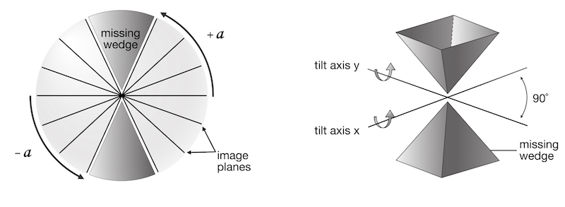
Since the collected tilt range does not cover a full 180°, there is a “missing wedge” of information when the 3D volume is calculated (ETFIG 2). Data close to the electron beam normal (corresponding to the 90° tilt angle) is missing and, as a result, tomograms will have anisotropic resolution (Baumeister and Steven, 2000). In the direction along the tilt axis (y), the resolution is limited to the nominal resolution of the microscope. In the direction perpendicular to the tilt axis (x), resolution is calculated by the equation above. In the z-direction, resolution is about half of the x resolution (or 2d as calculated above). To reduce the effects of the missing wedge, it is common to use dual-axis tomography (Mastronarde, 1997; Penczek et al., 1995), which decreases the missing wedge into a missing pyramid. This effectively increases the z-resolution to about 1.5 times the x-resolution (1.5d), and makes both the x and y resolutions the nominal resolution of the microscope. To do this, after collection of the first tilt series, the grid is rotated 90°, the ROI is re-found, and a second tilt series is collected.
Automation of Image Acquisition
Since each tilt series covers ~70-140 images, manually collecting images at various tilt angles would be tedious, particularly since following each tilt increment, the ROI needs to be aligned and refocused. Computer control of the image acquisition process automatically corrects image shifts and focus changes during acquisition of the tilt series. These procedures also minimize the electron dose on the sample during these adjustments. A commonly used automatic focusing technique calculates image movement between two images acquired at opposite beam tilts (Koster et al., 1987). Highly binned trial or tracking images are taken as the specimen is tilted, and these are used to keep the ROI aligned. By using the image shift coils of the microscope, alignment can be done very accurately, and more sloppy stage movements can be avoided. Tomographic data collection requires a well aligned microscope because of all of the image shifting and beam tilting required for data collection. In addition, there are several calibrations that need to be done on the automated software being used.
Besides automating tilt series collection, another key item is the capability to collect maps or montages. Within a “navigator” map, the ROI can be easily found and marked for automated collection. A map is essential for collecting dual axis tilt series. FEI provides its own software for its series of microscopes. Alternative software automation packages include Leginon (originally developed for automated single particle data acquisition) (Suloway et al., 2009; Amat et al., 2008) and SerialEM (Mastronarde, 2005). SerialEM is available for many modern microscopes and cameras, and provides a powerful interface for automated data collection. This program models the changes in image shifts and focus changes at the first few tilt angles to predict image movements for the remainder of the tilt series. By assuming that the sample follows a certain geometric rotation, the optical system characterizes the offset between the optical and mechanical axes. Thus, image movement in the x, y, and z directions due to stage tilt can be dynamically predicted with high accuracy. Based on experience with three microscopes (Tecnai F20; JEOL 2100; JEOL 3200FSC), full tomogram acquisition at 2° tilt increments using the Saxton scheme can be completed in one hour or less, making it possible to collect many tilt series in a given session on the microscope. This speed of acquisition becomes essential for collecting multiple tilt series across serial sections.
Image Alignment
In most automated image acquisition systems, shifts, rotations and magnification changes can occur during the specimen tilting process. Accurate alignment of projection images is essential for obtaining a high-quality tomographic reconstruction. For successful alignment, geometric relationships between the object of interest and the obtained projections need to be calculated. Ideally all image alignment defects should be corrected so that each image represents a projection of the same 3D object at the known projection angle. Inadequate image alignment will result in blurring or smearing of features in the reconstruction. Techniques have been developed to determine the geometric parameters for the sample throughout each projection angle or tilt increment.
External fiducial objects can be added to the sample before imaging in order to minimize drift of the ROI while calculating the tomogram. An alternative method called “markerless alignment” requires no external fiducial marks. Both methods have been used successfully for nematode tissues.
Fiducial Marker Alignment Methods
The coordinates of electron dense markers such as gold particles can be helpful to align a series of tilt images (Mastronarde, 2005; 2006). Fiducial markers have the advantage of being globally consistent in alignment among the images for the full range of tilt angles. The method can also be used to correct for anisotropic and non-uniform changes occurring to the specimen during the tilt series. Markers for plastic sections should be placed above and below the sample at a concentration such that a reasonable number (~10-30) are in the field of view when imaging the ROI.
Small gold beads are typically used in liquid suspension. A droplet is applied on one side of the microscope grid, and then blotted to remove excess liquid and allowed to air dry. A second droplet is next added to the second side of the grid and blotted again and allowed to dry prior to microscopy. Since the gold beads now lie on the outside surface of the section, they are convenient for following the exact motions of the ROI during tilt image collection. Despite overlying the ROI itself, the very thin projection planes of the final tomogram do not allow the gold markers to become visible within the viewing area of the tissue itself. They can be added to the grid before or after post-staining the sections.
Fiducial-less Alignment Methods
Methods have been developed for cases where markers cannot or have not been added. These generally are based on cross-correlation between successive images. The protomo software package (Winkler and Taylor, 2006) uses an iterative projection matching technique in which the full geometry of the sample in the microscope is determined. Besides lacking the requirement for fiducial markers, this software is scriptable since it uses only a command line interface. This makes automated simultaneous calculations of many tomograms on a computer cluster possible which is extremely useful for alignment of C. elegans tilt series of serial sections (for examples see ETFIG 3, ETFIG 4, ETFIG 5 & ETFIG 6).
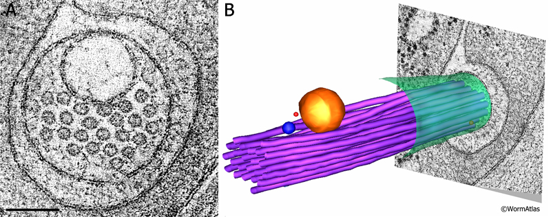
ETFIG 3: Electron tomogram of a touch dendrite. A. Raw image of ALM dendrite within the dual axis electron tomogram, face on, prior to any annotation. This is a mathematical model built after Fourier analysis, not a micrograph. Note that the microtubules are clustered near a large vesicle, which is likely cargo to be moved by microtubule-based motors inside the dendrite. HPF/FS sample. Image capture by KD Derr (NYSBC), Technai20 TEM. Tomogram calculated using weighted back projection from internal features by Bill Rice (NYSBC). Scale bar, 100 nm. B. Hand-annotated elements of the ALM dendrite and its neighborhood. Note that the microtubule bundle bends to accommodate passage of the vesicle. Purple, microtubules; red, ribosomes; yellow, large vesicle; blue, small vesicle; green, ALM plasma membrane. IMOD annotation by Kristin Politi (see Topalidou et al., 2012). This tomogram can also be viewed as a movie.
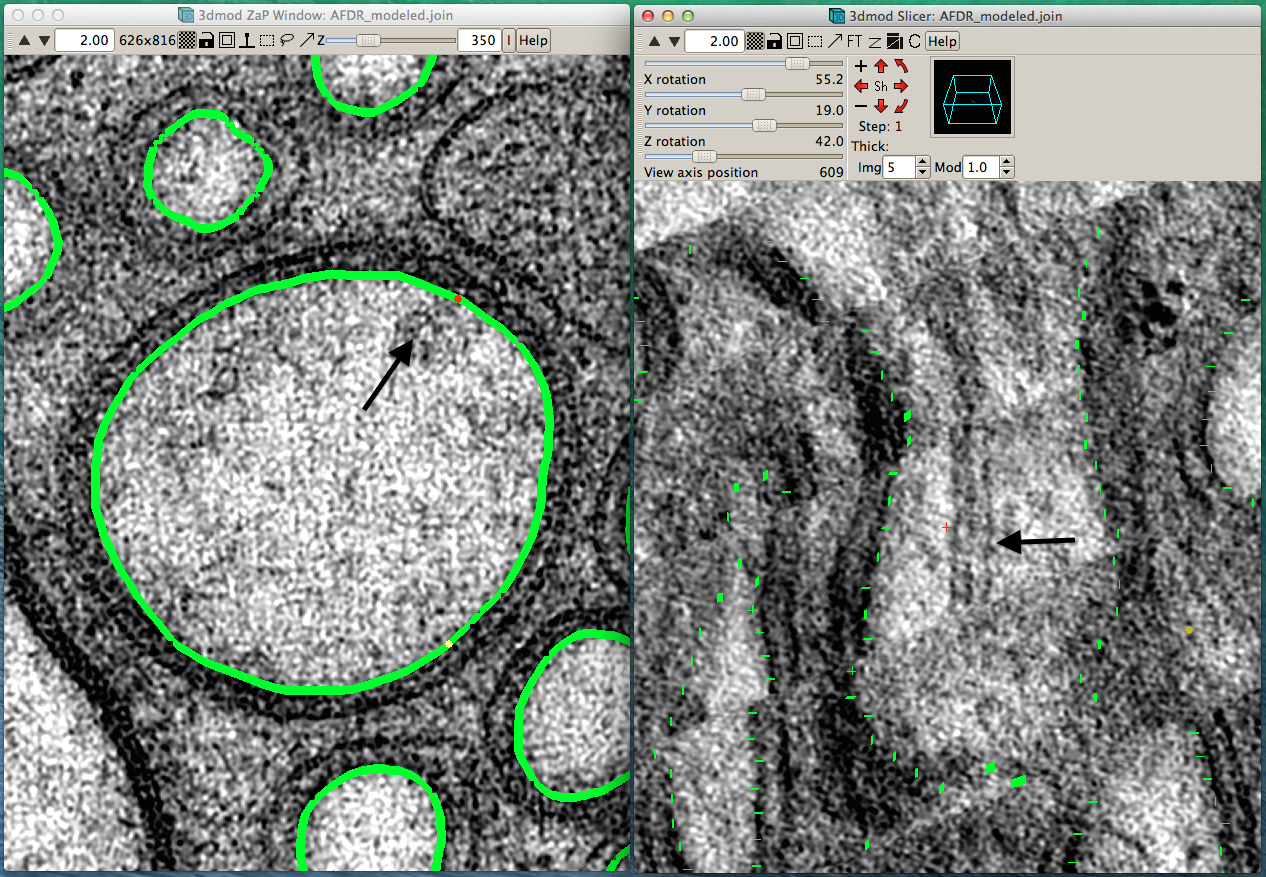
ETFIG 4: IMOD window with two views for annotation.
Sample working space in IMOD in which two projection planes of the same object can be seen at different angles to one another. Left panel. Distal dendrite of AFD is seen in “orthoslice” 350, with the main branches traced in green. Right panel. Same region is seen almost lengthwise, with faint green highlights marking outlines of cell processes. Arrows in each panel indicate the same object, a doublet microtubule. Tissue annotation by Emily Semaya.
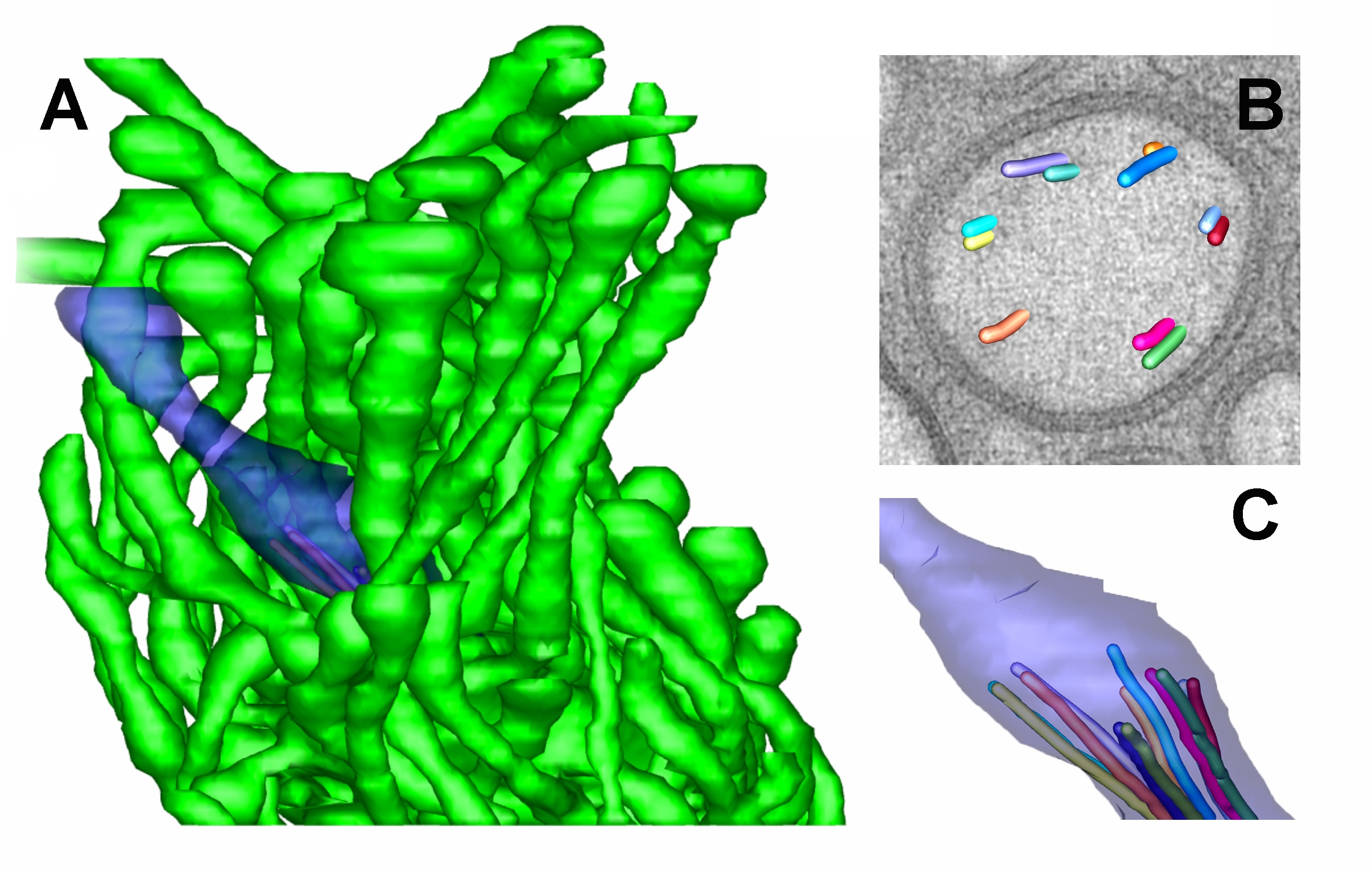
ETFIG 5: 3D model of AFD ending. A. Complex neuron ending of the AFD neuron include one short cilium (purple) and multiple microvilli (green) emerging from the dendrite tip. From a tomogram covering 15 serial sections. Scale bar is one micron. B. Closer view at the base of the cilium, where microtubules are shown extruding from one slice through the tomogram. Microtubules organize as doublets here, with almost no singlet microtubules extending distally beyond the axoneme. C. Individual microtubules of the cilium axoneme are modeled, showing that they all stop short, and do not enter the distal tip of the cilium. Microscopy conducted by Ken Nguyen and Willisa Liou. Tissue model created in IMOD by Emily Semaya.
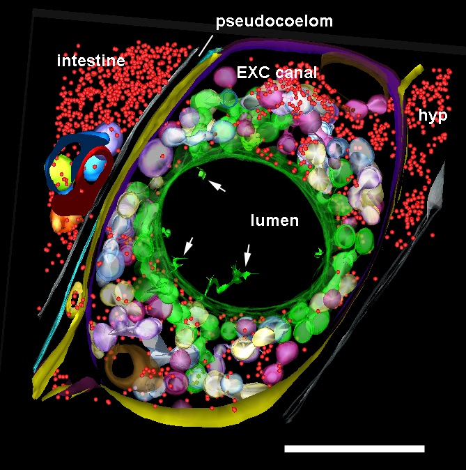
ETFIG 6: Annotated adult excretory canal. The complex physical relationships between the internal organelles of the excretory canal have been modeled within three semi-thin serial sections in a dual axis tomogram (cf. Khan et al., 2013). Despite the rather crowded nature of this tissue, the relationships among many smaller objects become much more visible in the tomogram compared to 50 nm thin sections, and simpler to annotate compared to a stack of serial TEM micrographs. Some features have only become apparent in the tomogram, such as the filamentous structures in the lumen (white arrows). Ribosomes, red; bead-like canaliculi, green, white and violet; outer plasma membrane of canal cell, yellow and purple; plasma membrane apposed to inner lumen, green. Nearby tissues include the hypodermis (hyp), intestine, and an expansion of the extracellular space, the pseudocoelom. Scale bar is one micron. Microscopy conducted by Ken Nguyen. Tissue model created in IMOD by Ashleigh Bouchelion.
3-D Tomogram Reconstruction
After having collected a tilt series with pre-determined tilt increments and specific angular assignments for each projection, an appropriate technique for 3D reconstruction needs to be chosen. There are three main methods used for 3D reconstruction: weighted back-projection, simultaneous iterative reconstruction technique (SIRT) (Gilbert, 1972), and algebraic reconstruction techniques (ART) (Radermacher, 2006). The first technique is the simplest and most commonly used while the latter two techniques require knowledge of several input parameters and are computationally expensive. However, SIRT is now commonly used, since programs such as IMOD provide a GUI, and allow calculations to be performed on a GPU (graphics card) to accelerate the process.
Back-projection Methods
Back-projection is a simple operation to understand, as it is the inverse of the projection operation. The 2D projections are smeared out by re-projecting them along the angles at which they were collected. By summing all of these re-projections, an estimate of the original object can be formed. However, this simple summation does not reconstruct the object exactly, since low resolution terms are overweighted and high-resolution terms are underweighted or undersampled. Therefore, a more faithful reproduction can be obtained by weighting the summation according to 1/r*, where r* is the distance from the origin in Fourier space (Radermacher, 2006). This modified algorithm is known as weighted back-projection. All of the tomographic software suites include a weighted back-projection reconstruction as a standard technique.
Algebraic and Iterative Methods
The ART and SIRT methods involve back-projection, re-projection of the newly constructed volume and then comparison with the original projections. This comparison allows for corrections in the re-projection algorithm. The main difference between ART and SIRT is that ART involves successive corrections whereas SIRT calculates simultaneous corrections of all projections. Unlike weighted back-projection, ART and SIRT are non-linear and require estimates of several correction parameters to begin, as well as limits for number of iterations and amount of allowable corrections. ART is available in TomoJ (Messaoudi et al., 2007). SIRT is available in TomoJ, the TOM Toolbox (Nickell et al., 2005), SPIDER (Frank et al., 1996) and IMOD (Kremer et al., 1996).
Filling in the Missing Wedge
After collecting one or more tilt series in the ROI, it is best to rotate the grid 90°, find the same ROI, and collect a second set of tilt series. The orthogonal data sets are then combined to reduce the missing wedge to a missing pyramid, and thus increase the signal to noise ratio of the final reconstruction. There are two strategies for combining the data: either all data is considered at once and combined to make a tomogram, or two separate tomograms are calculated then aligned and combined. The “all at once” method is implemented in SPIDER (Penczek et al., 1995), and more recently in protomo (Winkler and Taylor, 2013), while the merging method is available in IMOD (Mastronarde, 1997). As implemented in IMOD, the merging method works with and without fiducial markers, though more manual effort is required in samples without fiducials. In both cases, after an initial alignment, the second tomogram is “warped” to match the first tomogram, and this warping takes into account any additional shrinkage which has taken place during data collection. It is not clear which method is better, as different studies have found one or the other provided better results. This is likely sample dependent, with the merging method being better for samples that have more distortions in the second tilt series (Winkler and Taylor, 2013).
Note: We are currently using protomo to align our tilt series. For dual tilt series, each one is processed separately. We then use custom scripts to convert the protomo output into IMOD format, and use IMOD to merge the reconstructions manually. It takes a practiced user about 30 minutes to merge each tilt pair. We also generally convert the final maps to “byte” format, which not only reduces the file size but also ensures that density levels of stacked tomograms are the same.
Stacking Tomograms in Three Dimensions
Quite often, one semi-thick section is not enough to cover the volume of interest, and so (dual-tilt) tomograms are collected at corresponding ROIs of serial sections. Once the tomograms are calculated and merged, they are then stacked in three dimensions to produce a larger volume. This is easily done using the IMOD suite. One selects the series of tomograms to merge, making sure that the order is correct. Subsections are chosen from the top and bottom of each set, then aligned using a GUI and automated tools. One has the option to join using only rigid body movements (rotation and translation) or magnification change and stretching can also be taken into account. A final “joined” volume contains all of the aligned tomograms. It is important to note that this volume may be very large, since each individual volume is on the order of 2000x2000x150 voxels, and the final joined tomogram may be, for example, 10 times this size if 10 volumes were merged.
"Large" Tomograms
For even larger volumes, one may collect adjacent, overlapping ROIs and merge laterally. However, this is a somewhat difficult procedure, and it is easier to use the TEM collection software to collect “montage” tomograms that are more than one CCD frame in width. This is possible, for example, in SerialEM. One advantage of collecting with SerialEM is that IMOD software can automatically merge the individual frames from each part into a single larger image. However, for montages larger than 2X2 frames (at 2K x 2K pixels per frame), memory is an important consideration.
Calculating Tomogram Resolution
After reconstruction of a tomogram, how accurate is this model of the original structure? One criterion is the "resolution" of the tomogram: but what is meant by resolution? Resolution can be defined as the minimum distance by which two points can be separated and still identified as individual points (the point-to point resolution or Rayleigh criterion). In the case of ETs, this is not so useful since the resolution is anisotropic due to the missing wedge, or at best missing pyramid, in data collection (ETFIG 2). In the case of plastic sections, the z direction has been pre-shrunk by ~40% before data collection (Lucic et al., 2005). Additional factors such as the size of the stain particles (1-3 nm), and variations in staining and preservation, all add noise to the images. Finally, the thicker images collected at high tilt angles have more inelastic scattering and lower quality than un-tilted images. Therefore all projections do not contribute equally to the reconstruction. Finally, any errors in image alignment will lower the quality of the reconstruction. All of these factors cause the final resolution of the ET to be lower than any theoretical calculation based on tilt geometry. Calculation of resolution is not a trivial task, and while some methods have been proposed (Cardone et al., 2005; Unser et al., 2005), none are convenient to use or provide a simple number. In general, the resolution is best assessed by seeing the smallest features that can be reliably identified in the reconstructed volume, for example membrane bilayer structure or mitochondrial cristae.
Reducing Tomogram Noise
The amount of noise in the tomogram makes a simple surface view of the 3D volume nearly impossible to interpret, and also makes it difficult to identify features. Various filters can be applied to improve the signal to noise ratio in the tomogram. The simplest filter to apply is a low-pass filter, which will enhance contrast by removing high frequency information mostly likely caused by noise. This could be applied with a soft cutoff at the maximum resolution determined above. While easy to perform, this sort of filter does not discriminate between signal and noise, and so real data is discarded. A better alternative is to apply a median filter, a real-space filter in which adjacent pixels are fixed to their median value. The median filter tends to enhance features, and can produce more satisfying results than the low-pass filter. It is relatively fast and can be applied consecutively, though again it does not discriminate between signal and noise.
Advanced noise filtering methods have been developed for image post-processing which are designed to decipher the signal and separate it from the noise. These include non-linear anisotropic diffusion (NAD) (Frangakis and Hegerl, 2001; Fernandez and Li, 2003) and a non-local means filter implemented in Amira software (Stalling et al., 2005). These filters all tend to enhance edges in the data while reducing the background noise level. This more advanced filtering requires much higher computational cost. In addition, they all have several parameters that much be specified. In general these parameters are dataset specific, and must be found by trial and error. For plastic sections, we have found that median filters are often sufficient to aid segmentation, and we go to the other filters only when needed.
Tomogram Annotation
The final step in electron tomography is interpreting the tomogram itself. If the tomogram does not consist of several repeating motifs, then one must label and identify different features in the tomogram. This annotation process is often called “segmentation” (see ETFIG 3, ETFIG 4, ETFIG 5 & ETFIG 6). Resolving individual components within a tomogram is a very difficult and time-consuming process due to the low signal-to-noise ratio and the volume of data within the tomogram. In general, segmentation is done on filtered volumes, as raw tomograms are very difficult to segment. Most segmentation to date has been done manually, using software packages such as IMOD (Kremer et al., 1996) or Amira (Stalling et al., 2005). With these programs, the user goes slice-by-slice through the tomogram and manually paints the different features. Amira includes options such as selection by intensity and interpolation to speed up the process, and also has automated techniques for segmenting some cellular features such as microtubules. Both packages allow different orientations to be viewed (xy, xz, yz) and allow many objects to be created (ETFIG 4). As can be imagined, annotation can be a very labor intensive process, but the final results can be striking (Müller-Reichert et al., 2003; Stigloher et al., 2011; Topalidou et al., 2012; Doroquez et al., 2014). The TomoJ plugin module for ImageJ is another practical choice for segmentation (Messaoudi et al., 2007).
Notes:
A tomogram will contain information about three dimensional structures that can be examined from any angle. The “orthoslice” is a projection image of the ET at a given depth along the z axis, coincident with the original viewing angle of the thin sections (left panel in ETFIG 4). However, by re-slicing the ET at a new angle, one can bring structures into optimal view, no matter what orientation the object had in the original slices (right panel in ETFIG 4). While a spherical object like a small vesicle should look rather similar from any viewing angle, a microtubule or myelin rod will be much better viewed when exactly orthogonal to its main axis or exactly lengthwise (ETFIG 5). For the time being, annotation must generally be performed by hand at the computer monitor, tracing portions of the cells and organelles using a computer mouse, or using a stylus on a touchscreen or a drawing tablet, such as the Wacom Cintiq display.
We use the Amira software package to produce Quicktime movies from our IMOD-based tomogram models. Amira provides much creative freedom in switching between movies of the orthoslices, and extrusion of the modeled cells and organelles. Additional examples of IMOD models and Amira-based Quicktime movies from our work on C. elegans can be viewed at http://www.wormatlas.org/movies.htm
Software Tools
The IMOD software suite (Kremer et al., 1996) provides methods for fiducial and fiducial-free alignments and calculates reconstructions by back-projection or SIRT. It also provides means to merge tilt pairs and stack serial tomograms. It offers a complete suite for all methods and has a graphical user interface (GUI) for most techniques. The SPIDER software suite (Frank et al., 1996) also contains a set of scripts for alignment and reconstruction of tomograms. The protomo software suite (Winkler and Taylor, 2013) is mostly run through a set of command line scripts and programs, and provides means for fiducial-free alignment and reconstruction. We use a series of scripts to batch submit tomograms to a computer cluster for processing by protomo. Other software packages used for tomographic reconstructions include RAPTOR (for automated alignment of fiducials) (Amat et al., 2008), the TOM Toolbox (a Matlab extension) (Nickell et al., 2005) and TomoJ (a plugin for ImageJ) (Messaoudi et al., 2007). Newer tomogram analysis tools are also being developed using FIJI as the platform of choice (Irobalieva et al., 2016).
For more information, see Computer-Based Analytical Tools.
References
Amat, F., Moussavi, F., Comolli, L.R., Elidan, G., Downing, K.H. and Horowitz, M. 2008. Markov random field based automatic image alignment for electron tomography. J. Struct. Biol. 161: 260-275. Abstract
Baumeister, W. and Steven, A.C. 2000. Macromolecular electron microscopy in the era of structural genomics. Trends Biochem. Sci. 25: 624-631. Abstract
Cardone, G., Grunewald, K. and Steven, A.C. 2005. A resolution criterion for electron tomography based on cross-validation. J. Struct. Biol. 151: 117-129. Abstract
Crowther, R.A., Amos, L.A., Finch, J.T., De Rosier, D.J. and Klug, A. 1970. Three dimensional reconstructions of spherical viruses by Fourier synthesis from electron micrographs. Nature 226: 421-425. Abstract
Doroquez, D.B., Berciu, C., Anderson, J.R., Sengupta, P. and Nicastro, D. 2014. A high-resolution morphological and ultrastructural map of anterior sensory cilia and glia in Caenorhabditis elegans. eLife 3: e01948. Article
Egerton, R.F., Li, P. and Malac, M. 2004. Radiation damage in the TEM and SEM. Micron 35:399-409. Abstract
Frangakis, A.S. and Hegerl, R. 2001. Noise reduction in electron tomographic reconstructions using nonlinear anisotropic diffusion. J. Struct. Biol. 135: 239-250 Abstract
Frank, J., Radermacher, M., Penczek, P., Zhu, J., Li, Y., Ladjadj, M. and Leith, A. 1996. SPIDER and WEB: processing and visualization of images in 3D electron microscopy and related fields. J. Struct. Biol. 116: 190-199. Abstract
Gilbert, P.F.C. 1972. The reconstruction of a three-dimensional structure from projections and its application to electron microscopy. II. Direct methods. Proc. R. Soc. Lond. B 182: 89-102. Abstract
Hall, D.H. and Rice, W.J. 2015. Electron tomography mehtods for C. elegans. Methods Mol. Biol. 1327: 141-58. Abstract
Hall, D.H., Hartweig, E. and Nguyen, K.C.Q. 2012. Modern electron microscopy methods for C. elegans. Methods Cell Biol. 107: 93-149. Abstract
Irobalieva, R.N., Martins, B. and Medalia, O. 2016. Cellular structural biology as revealed by cryo-electron tomography. J. Cell Sci. 129: 469-76. doi: 10.1242/jcs.171967. Article
Lucic, V., Forster, F. and Baumeister, W. 2005. Structural studies by electron tomography: from cells to molecules. Annu. Rev. Biochem. 74: 833-865. Article
Luther, P.K., Lawrence, M.C. and Crowther, R.A. 1988. A method for monitoring the collapse of plastic sections as a function of electron dose. Ultramicroscopy 24: 7-18. Abstract
Koster, A.J., van der Bos, A. and van der Mast, K.D. 1987. An autofocus method for TEM. Ultramicroscopy 21: 209-222. Article
Kremer, J.R., Mastronarde, D.N. and McIntosh, J.R. 1996. Computer Visualization of Three-Dimensional Image Data Using IMOD. J. Struct. Biol. 116: 71–76. Abstract
Mastronarde, D.N. 1997. Dual-axis tomography: an approach with alignment methods that preserve resolution. J. Struct. Biol. 120: 343-352. Abstract
Mastronarde, D.N. 2005. Automated electron microscope tomography using robust prediction of specimen movements. J. Struct. Biol. 152: 3651. Abstract
Mastronarde, D.N. 2006. Fiducial marker and hybrid alignment methods for single- and double-axis tomography. In Electron Tomography: Methods for three-dimensional visualization of structures in the cell. Frank J (ed). 2nd edition. Springer, New York. pp.163-186. Abstract
Messaoudi, C., Boudier, T., Sorzano, C.O.S. and Marco, S. 2007. TomoJ: tomography software for three-dimensional reconstruction in transmission electron microscopy. BMC Bioinform. 8: 288-297. Article
Müller-Reichert, T., Hohenberg, H., O’Toole, E.T. and McDonald, K.L. 2003. Cryoimmobilization and three-dimensional visualization of C. elegans ultrastructure. J. Microsc. 212:71-80. Article
Nickell, S., Forster, F., Linaroudis, A., Net, W.D., Beck, F., Hegerl, R., Baumeister, W. and Plitzko, J.M. 2005. TOM software toolbox: acquisition and analysis for electron tomography. J. Struct. Biol. 149: 227-234. Abstract
Penczek, P., Marko, M., Buttle, K. and Frank. J. 1995. Double-tilt electron tomography. Ultramicroscopy 60: 393-410. Abstract
Radermacher, M. 2006. Weighted back-projection methods. In Frank J (ed) Electron Tomography: Methods for three-dimensional visualization of structures in the cell. 2nd edition. Springer, New York. pp.245-27. Abstract
Saxton, W.O., Baumeister, W. and Hahn, M. 1984. Three-dimensional reconstruction of imperfect two-dimensional crystals. Ultramicroscopy 13: 57-70. Abstract
Stalling, D., Westerhoff, M. and Hege, H.-C. 2005. Amira: A highly interactive system for visual data analysis. In: Hansen, C.D. and Johnson, C.R. (eds) The Visualization Handbook, Elsevier, London, pp. 749-787. Article
Stigloher C., Zhan, H., Zhen, M., Richmond, J. and Bessereau, J.L. 2011. The presynaptic dense projection of the Caenorhabiditis elegans cholinergic neuromuscular junction localizes synaptic vesicles at the active zone through SYD-2/Liprin and UNC-10/RIM-dependent interactions. J. Neurosci. 31:4388-96. Article
Suloway, C., Shi, J., Cheng, A., Pulokas, J., Carragher, B., Potter, C.S., Zheng, S.Q., Agard, D.A. and Jensen, G.J. 2009. Fully automated, sequential tilt-series acquisition with Leginon. J. Struct. Biol. 167: 11-18. Article
Topalidou, I., Keller, C., Kalebic, N., Nguyen, K.C., Somhegyi, H., Politi, K.A., Heppenstall, P., Hall, D.H. and Chalfie, M. 2012. Genetically separable functions of the MEC-17 tubulin acetyltransferase affect microtubule organization.
Curr. Biol. 22:1057-65. Article
Unser, M., Sorzano, C.O., Thevenaz, P., Jonic, S., El-Bez, C., De Carlo, S., Conway, J.F. and Trus, B.L. 2005. Spectral signal-to-noise ratio and resolution assessment of 3D reconstructions. J. Struct. Biol. 149: 243-255. Article
Winkler, H. and Taylor, K.A. 2006. Accurate marker-free alignment with simultaneous geometry determination and reconstruction of tilt series in electron tomography. Ultramicroscopy 106: 240–254. Abstract

Edited for the web by Laura A. Herndon. Last revision: August 3, 2017
|